Author: Romain Vergne (
website)
Please cite my name and add a link to my web page if you use this course
Image synthesis and OpenGL: lighting
Quick links to:
- The
problem
- Color
- The
rendering equation
- Local
lighting
- Types
of lights
- Types
of reflections
- Computing
lighting on the GPU
- Sources
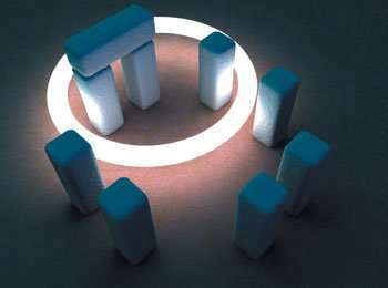
The problem
|
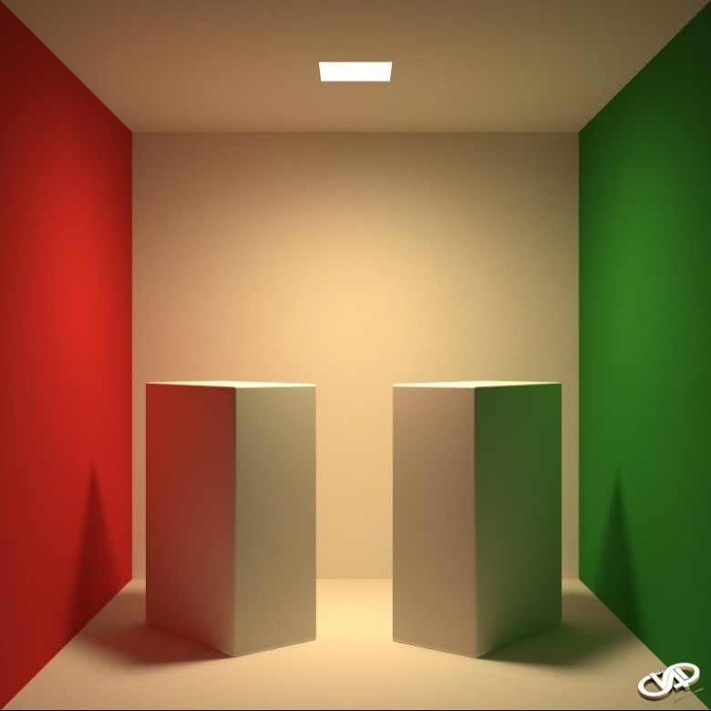
The illumination on a given point of the surface depends on:
- primary light sources
- secondary light sources
- all the objects in the scene
- an illuminated object becomes a light source
- indirect lighting
Cornel box (1984)
|
We will be mainly interested in direct
lighting and local illumination in this course.
|
The illumination on a given point of the surface depends on:
- The viewpoint
- The surface properties
- reflexion
- absorption
- diffusion
- The light properties
- direction
- wavelenght
- energy
Involve
a lot of dimensions
|
Color
Physically, visible light is an electromagnetic wave
|
|
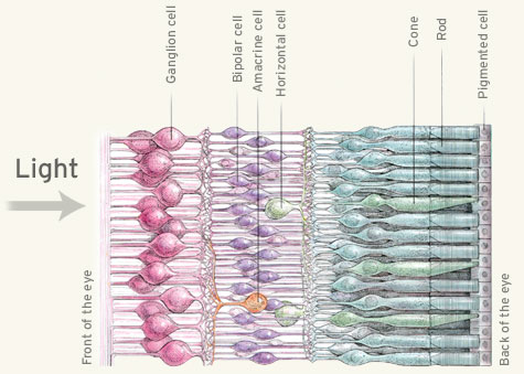
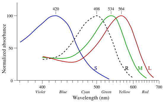
| Physiologically,
our eyes use 3 types of sensors to perceive light colors |
In computer science
 |

|
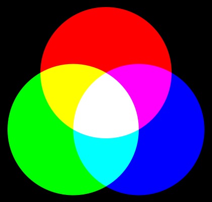
Additive models
(lighting)
|
Soustractive
models
(painting)
|
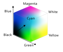
- RGB(A) for
Red, Green, Blue (Alpha) is the most well known additive model
- Easy to use in graphics applications
- Difficult to ensure the same color on different screen...
(gamut)
- CIE
1931 XYZ color space
- The tristimulus values can be conceptualized as amounts of
three primary colors in a trichromatic additive color model.
- The CIE (Comission Internationale
de l'éclairage) was the first to mathematically define a
trichromatic system to represent perceived colors.
- It is based on the standard (colorimetric) observer and
thus allows to uniquely represent colors in a 3D space.
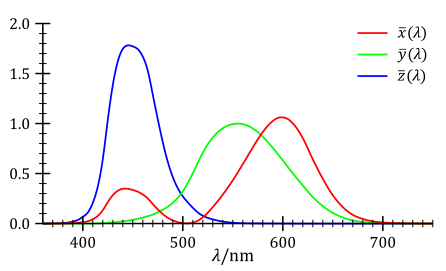
Color matching functions: spectral
sensitivity
curves of 3 linear light detectors
|
If \( I (\lambda) \) is the spectral
distribution of a color, then:
\[
X = \int_{400}^{800} I(\lambda) \bar{x}(\lambda) d \lambda
\]
\[
Y = \int_{400}^{800} I(\lambda) \bar{y}(\lambda) d \lambda
\]
\[
Z = \int_{400}^{800} I(\lambda) \bar{z}(\lambda) d \lambda
\]
|
- CIE Yxy
color space
- Normalize the XYZ color space and decompose it into Luminance (Y)
and chrominance (xy)
- CIE
Lab color space
- Perceptually uniform: distance between 2 colors = perceived distance
between these colors
- Used in most graphics applications
- L = luminance
- a = chrominance (red-green)
- b = chrominance (blue-yellow)
- HSV (Hue,
Saturation, Value) color space
- In most image processing software: Photoshop, Gimp, etc.
- Intuitive for designers
- CMY(K),
for Cyan, Magenta, Yellow (and Key - Black)
- Subtractive model
- Mainly used for printing
- ETC....: Adobe RGB, sRGB, CIELuv, CIEUvw, YIQ (NTSC), YUV (PAL), HSL,
....
|
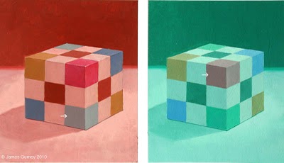
Still, the perception of colors is
not well understood and the perfect color space does not exist!
(example of color contrast)
try this excellent
demo
|
Coding colors
- Binary representation: 0 or 1
- 8 bits: 0 to 255 grey levels (monochromatic)
- 24 bits: 8 bits per channel (polychromatic)
- 256 values per channel (usually RGB)
- 256*256*256 = 16 777 216 colors
- limited: 8 orders of magnitude between the sun and stars
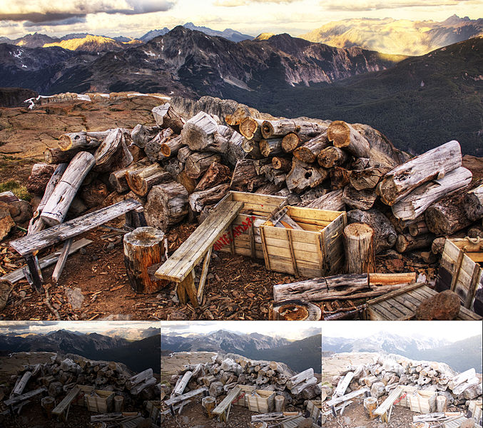
- HDR (High Dynamic Range) images: float or double precision per channel
- 24 bits per channel = \( 256^9 \) colors
- Can be created using multiple LDR (Low Dynamic Range) images
- Needs to be tonemapped to be displayed on a screen
The rendering
equation [Kajiya
1986]
\[
L(\mathbf{p} \rightarrow \mathbf{e}) =
L_e(\mathbf{p} \rightarrow \mathbf{e}) +
\int_{\Omega_\mathbf{n}}
\rho(\mathbf{p}, \mathbf{e}, \pmb{\ell})
(\mathbf{n}\cdot\pmb{\ell}) \
L(\mathbf{p} \leftarrow \pmb{\ell}) \
d\pmb{\ell}
\]
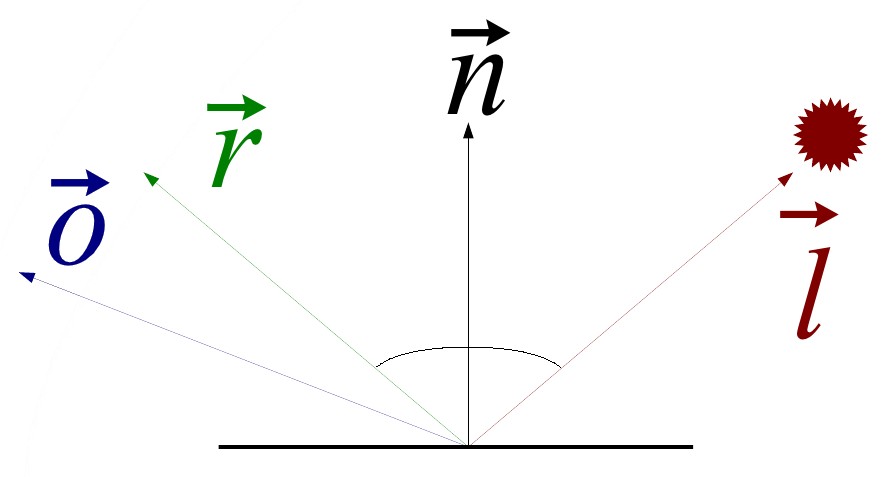
- \( \mathbf{p} \) is a point on the surface
- \( \mathbf{e} \) is the view direction
- \( \mathbf{n} \) is the normal of the surface at point \( \mathbf{p}
\)
- \( \pmb{\ell} \) is the direction of a light in the hemisphere \(
\Omega_\mathbf{n} \)
- \( L(\mathbf{p} \rightarrow \mathbf{e}) \):
- outgoing radiance (in \( Wm^{-2}sr^{-1}) \)
- how much energy is arriving to the eye / camera
- \( L_e(\mathbf{p} \rightarrow \mathbf{e}) \):
- emitted radiance
- usually equal to 0 for object surfaces (they do not create energy)
- \( L(\mathbf{p} \leftarrow \pmb{\ell}) \):
- incoming radiance
- incident illumination leaving the light \( \pmb{\ell} \) and
arriving at the point \( \mathbf{p} \) of the surface
- \( (\mathbf{n}\cdot\pmb{\ell}) \):
- the orientation of the surface
- dot product between \( \mathbf{n} \) and \( \pmb{\ell} \)
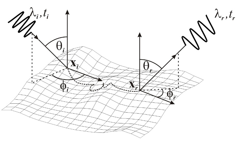
- \( \rho(\mathbf{p}, \mathbf{e}, \pmb{\ell}) \):
- material properties / BRDF (Bidirectional Reflectance Distribution
Function)
- how much energy the surface reflects in the viewing direction \(
\mathbf{e} \) given the incident light \( \pmb{\ell} \)
Local lighting
General equation
Empirical model for
computing the outgoing radiance
\[
L(\mathbf{p} \rightarrow \mathbf{e}) =
\rho_a L_a +
\sum_{k}
\rho(\mathbf{p}, \mathbf{e}, \pmb{\ell}_k) \
(\mathbf{n}\cdot\pmb{\ell}_k) \
L(\mathbf{p} \leftarrow \pmb{\ell}_k)
\]
- \( L(\mathbf{p} \rightarrow \mathbf{e}) \): outgoing radiance / light
energy / color
- \( \rho_a L_a \): ambient lighting (approximate indirect lighting)
- \( \sum_{k} \cdots \): contribution of each light \( \pmb{\ell}_k \)
- \(
\rho(\mathbf{p}, \mathbf{e}, \pmb{\ell}_k) \): BRDF - how the light
\( \pmb{\ell}_k \) is reflected on top of the surface
- \( (\mathbf{n}\cdot\pmb{\ell}_k) \): surface orientation (according to
light \( \pmb{\ell}_k \) )
- \( L(\mathbf{p} \leftarrow \pmb{\ell}_k) \): incoming radiance for
light \( \pmb{\ell}_k \)
The simplest model: assign a color at each point of the surface (albedo)
\[
L(\mathbf{p} \rightarrow \mathbf{e}) = color
\]
- Reflecting power of the surface
- Independent of the view direction
- Independent of the light direction
- Too simple:
- adapted for static scenes (photos) but not for dynamic ones (image
synthesis)
- dynamic viewpoint?
- dynamic lighting variations?
The second simplest model: consider a single dynamic light
\[
L(\mathbf{p} \rightarrow \mathbf{e}) =
\rho(\mathbf{p}, \mathbf{e}, \pmb{\ell}) \
(\mathbf{n}\cdot\pmb{\ell}) \
L(\mathbf{p} \leftarrow \pmb{\ell})
\]
- Which types of lights?
- Which types of surface reflections?
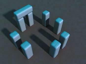
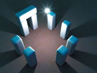
Types of lights
Infinitesimal
lights
|
|

|
|
Directionnal light
- Distant sources (sun)
- Environment maps (video-games)
\[
L(\mathbf{p} \leftarrow \pmb{\ell}) = L
\]
|
Point light
- position in space \( \mathbf{p}_{\pmb{\ell}} \)
- near, small sources
\[
L(\mathbf{p} \leftarrow \pmb{\ell}) = L/r^2
\]
with \( r = || \mathbf{p} -
\mathbf{p}_{\pmb{\ell}} || \) and \( \pmb{\ell} = \frac{\mathbf{p}
- \mathbf{p}_{\pmb{\ell}} }{r} \)
|
Spot light
- position in space
- near, small sources
- defined in a cone
- direction \( \mathbf{s}_{\pmb{\ell}} \)
- exponent \( e \)
- a cutoff \( c \)
\[
L(\mathbf{p} \leftarrow \pmb{\ell}) =
\frac{(\mathbf{s}_{\pmb{\ell}} \cdot \pmb{\ell})^e L}{r^2}
\]
if \( (\mathbf{s}_{\pmb{\ell}}
\cdot \pmb{\ell})<c \) and 0 otherwise
|
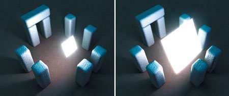
Area
lights
|
|
- Defined on volumes / surfaces
- Soft shadows
- Expensive!
|
Types of reflections
Lets consider a (white) directional light ( \( L=cst=(1,1,1) \) ). The model
is equal to:
\[
L(\mathbf{p} \rightarrow \mathbf{e}) =
\rho(\mathbf{p}, \mathbf{e}, \pmb{\ell}) \
(\mathbf{n}\cdot\pmb{\ell})
\]
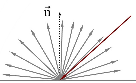
The lambertian model
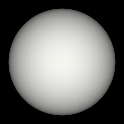
|
|
Lambertian
surface
|
\[ \rho(\mathbf{p}, \mathbf{e},
\pmb{\ell}) = cst \]
- Light is diffused in every direction
- Independant on the point of view
|
\[
L(\mathbf{p} \rightarrow \mathbf{e}) =
\rho_d \
(\mathbf{n}\cdot\pmb{\ell}) L_d
\]
|
\[
L(\mathbf{p} \rightarrow \mathbf{e}) =
\sum_k \rho_{kd} \
(\mathbf{n}\cdot\pmb{\ell}) L_{kd}
\] |
|
One light:
- \( \rho_d = \) constant diffuse material color
- \( L_d = \) constant diffuse light color
|
Multiple light
- sum of contribution of each light
- may have different color coeficients
|
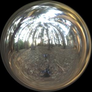
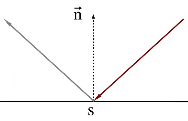
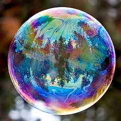
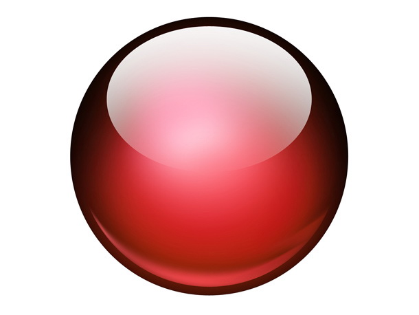
The mirror and transparent models
|
|
Mirror surface
|
\[ \rho(\mathbf{p}, \mathbf{e},
\pmb{\ell}) = cst\ if\ (\mathbf{r}\cdot\mathbf{e}=1),\ 0\ otherwise
\]
- Reflected light vector \( \mathbf{r}=2 \mathbf{n}
(\mathbf{n}\cdot \pmb{\ell})-\pmb{\ell} \)
- Dependant on the point of view
- Usefull for environment maps
- compute the reflected view vector
- \( \mathbf{r}=2 \mathbf{n} (\mathbf{n}\cdot
\mathbf{e})-\mathbf{e} \)
- use it to fetch a color in the map
|
|
|
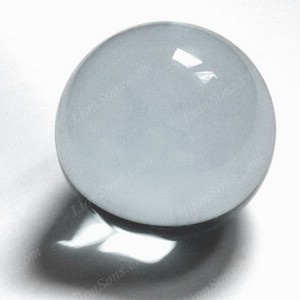
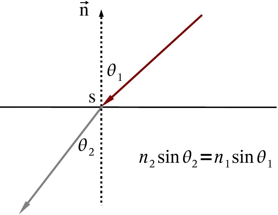
Transparent
surface
|
\[ \rho(\mathbf{p}, \mathbf{e},
\pmb{\ell}) = cst\ if\ (\mathbf{r}\cdot\mathbf{e}=1),\ 0\
otherwise \]
- Refracted
light vector \( \mathbf{r}=e \pmb{\ell} - (e (\mathbf{n}\cdot
\pmb{\ell}) + \sqrt{1-e^2 (1-(\mathbf{n}\cdot \pmb{\ell})^2)})
\mathbf{n} \)
- Dependant on the point of view
- Same principle for environment maps
|
\[
L(\mathbf{p} \rightarrow \mathbf{e}) =
\rho_s(\mathbf{p}, \mathbf{e}, \pmb{\ell}) \
(\mathbf{n}\cdot\pmb{\ell}) L_s
\]
|
\[
L(\mathbf{p} \rightarrow \mathbf{e}) =
\sum_k \rho_{ks} (\mathbf{p}, \mathbf{e}, \pmb{\ell})\
(\mathbf{n}\cdot\pmb{\ell}) L_{ks}
\] |
|
One light:
- \( \rho_s = \) constant specular material color
- \( L_s = \) constant specular light color
|
Multiple light
- sum of contribution of each light
- may have different color coeficients
|
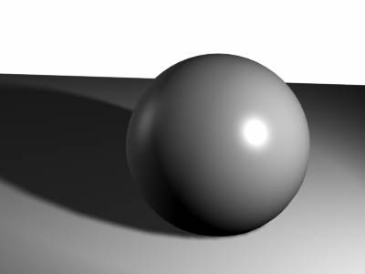
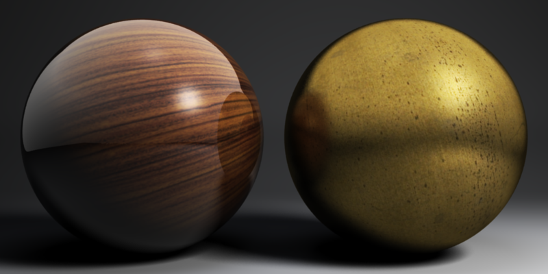
Glossy models
|
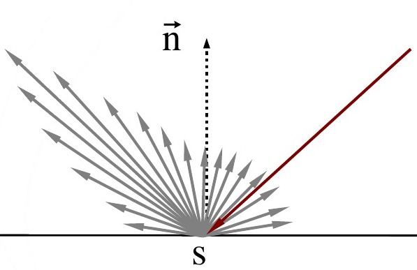
|
| Glossy surface |
\[ \rho(\mathbf{p}, \mathbf{e},
\pmb{\ell}) = \rho_d(\mathbf{p}, \mathbf{e}, \pmb{\ell}) +
\rho_s(\mathbf{p}, \mathbf{e}, \pmb{\ell}) \]
- Usually expressed as a sum of diffuse and specular terms
- \( \rho_d = cst \) (as before)
- \( \rho_s = (\mathbf{r}\cdot\mathbf{e})^e\) (for instance)
|
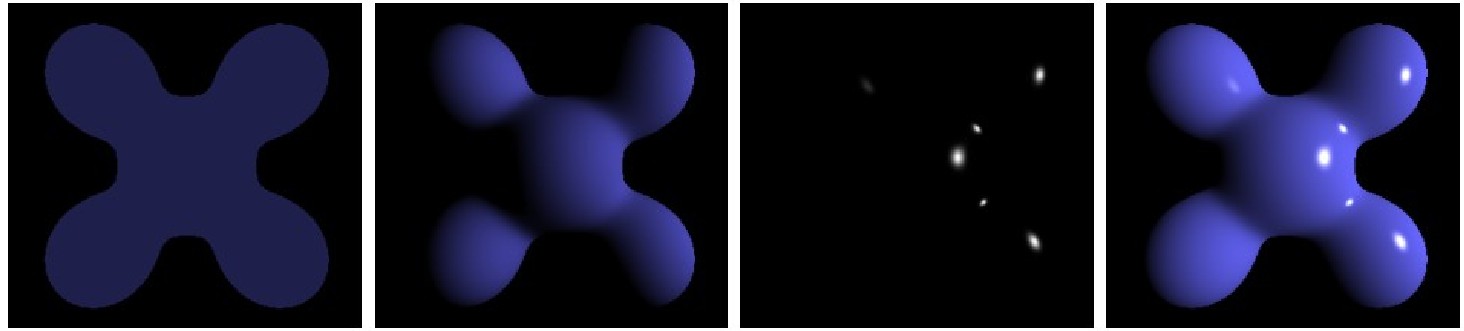
The Phong model
\( \rho_s =
(\mathbf{r}\cdot\mathbf{e})^e\)
The general formulation of the Phong model is given by a weighted sum of an
ambient, diffuse and specular term:
\[
L(\mathbf{p} \rightarrow \mathbf{e}) = \rho_a L_a + \sum_k
\rho_{kd} L_{kd} (\mathbf{n}\cdot\pmb{\ell}) + \rho_{ks} L_{ks}
(\mathbf{r}\cdot\mathbf{e})^e
\]
where
- \( \rho_a \), \( \rho_{kd} \) and \( \rho_{ks} \) are the
material colors for the ambient, diffuse and specular term,
respectively.
- \( L_a \), \( L_{kd} \) and \( L_{ks} \) are the light colors for the
ambient, diffuse and specular term, respectively.
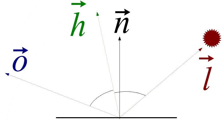
The Blinn-Phong Model
Specular term replaced by \(
\rho_s = (\mathbf{h}\cdot\mathbf{n})^e \) , with \(
\mathbf{h}=\frac{\pmb{\ell}+\mathbf{e}}{|| \pmb{\ell}+\mathbf{e}||} \)
Anisotropy effect
Specular term replaced by \( \rho_s =
(\mathbf{h}\cdot\mathbf{n})^{n_u cos^2\phi + n_v sin^2 \phi} \)
Fresnel effect
Obtained using Schlick approximation:
\( F = R_s + (1-R_s)(1-\mathbf{e}\cdot\mathbf{h})^5 \)
Other effects?
|
|
|
Diffraction
|
Non-realistic
effects
|
Varying material
properties
|
- Plenty of BRDFs (they are specialized for certain kinds of materials)
- Lambertian
- Phong
- Blinn-Phong
- Torrance-Sparrow
- Cook-Terrance
- Ward
- Oren-Nayar
- Ashikhmin-Shirley
- Lafortune
- etc...
- And also SVBRDF (for spatially varying BRDF)
- material parameters change over the surface (usually using textures
- And also BSSRDF (for Bidirectionnal Subsurface Scatering Distribution
Function)
- specific for translucent materials
- More generally: BXDF for Bidirectionnal X Distribution Function
How to compute
lighting on the GPU?
Flat shading
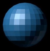
|
Compute lighting per face
- In the vertex shader
- Normals are constant for the vertices of each triangle
- Produce shading discontinuities
|
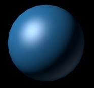
Gouraud Shading
 |
Compute lighting per vertex
- In the vertex shader
- Normals are different for each vertex
- Color is computed and interpolated during rasterization
- Quality / result depends on tesselation
|
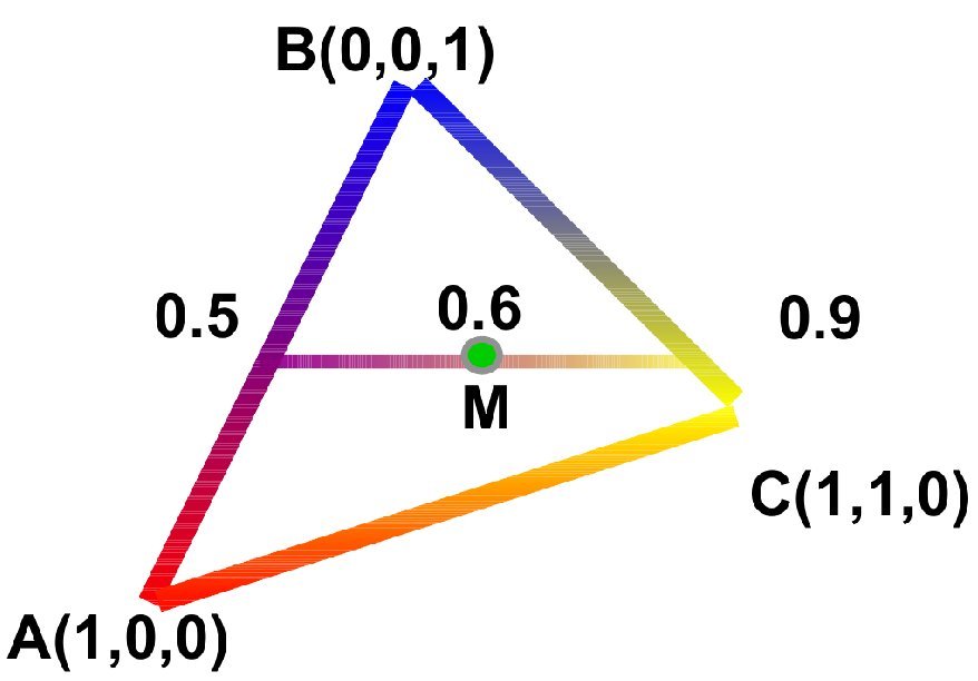
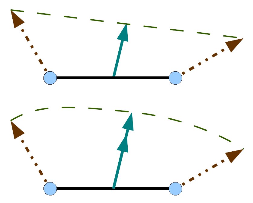
Question: what is the color at point
M?
|
Phong Shading (different from the Phong
model)
|
Compute lighting per fragment
- Normals are interpolated during rasterization (vertex to
fragment)
- Normals are re-normalized
- Color is computed
|
|
Sources